Sharpe Ratio: A "Lens" for Quantifying Risk and Performance in Real-World Investments

✍️By Thanh Ho

•

📅May 18, 2026

In a volatile financial market, sky-high returns are always a magnet for attention. However, is a 30% return truly superior to a 15% return if it comes at the cost of devastating asset declines? To answer this core question, fund managers and professional investors don't just look at the flashy growth figures; they use a special "lens": the Sharpe Ratio. Built on the foundation of Modern Portfolio Theory and honored with the prestigious Nobel Prize, this ratio is a mathematical bridge between return and risk.

1. Definition of the Sharpe Ratio

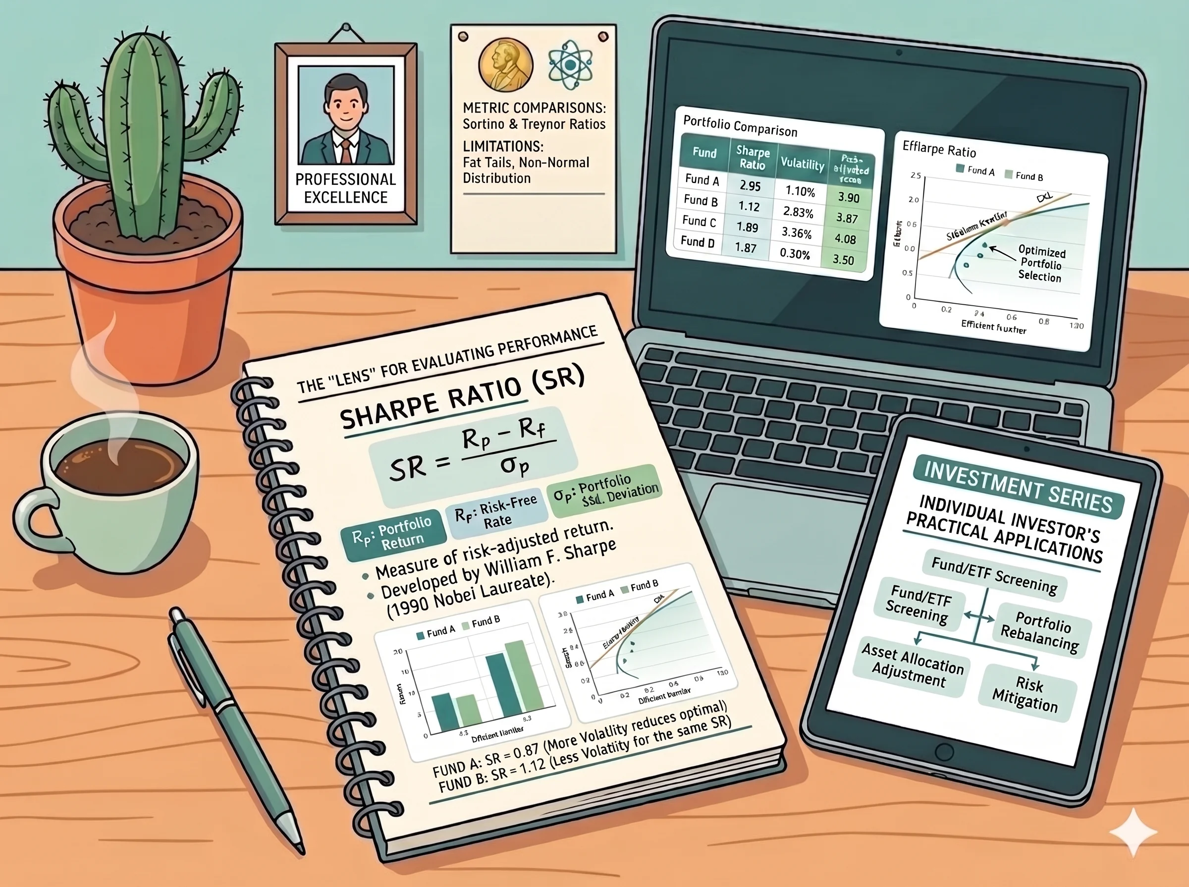
The Sharpe Ratio (Sharpe coefficient) is a financial performance metric used to evaluate the return earned per unit of risk for an investment portfolio or an individual asset. Simply put, the Sharpe Ratio helps investors answer the core question: "Given the level of risk I am enduring, is the excess return earned truly worth it?". A higher ratio indicates superior portfolio management efficiency, meaning that the investor achieves high returns without facing an excessively large degree of volatility.

2. History of the Sharpe Ratio

The Sharpe ratio was originally proposed by American economist William F. Sharpe in 1966 under its initial name, the "reward-to-variability ratio" (the ratio of reward over volatility).

Historical Context: The 1960s was a period when Harry Markowitz's Modern Portfolio Theory (MPT) was actively shaping and redefining global financial thinking.
The Objective: William Sharpe (a student of Markowitz) wanted to create a simple yet powerful tool to operationalize the measurement of risk-adjusted portfolio performance.
The 1994 Improvement: In 1994, William Sharpe published an updated article regarding the definition and calculation formula of this metric, officially renaming and standardizing it as the Sharpe Ratio we use today.
A Prestigious Award: Thanks to these monumental contributions—particularly the Capital Asset Pricing Model (CAPM) and the Sharpe Coefficient—William F. Sharpe was awarded the Nobel Prize in Economics in 1990.

3. Formula and Components of the Sharpe Ratio

3.1. Calculation Formula

The Sharpe Ratio is calculated based on the following mathematical formula:

$S R = \frac{R _{p} - R _{f}}{σ _{p}}$

Where:

$S R$ : The Sharpe Ratio metric.
$R_{p}$ (Portfolio Return): The expected (or actual) rate of return of the investment portfolio within a specific timeframe.
$R_{f}$ (Risk-free Rate): The risk-free rate of return. This represents the minimum return an investor can achieve with virtually zero risk of capital loss (typically derived from short-term or medium-term government bond yields of matching maturities).
$σ_{p}$ (Standard Deviation of Portfolio): The standard deviation of the portfolio's rate of return, representing the total risk (or risk volatility level) of that portfolio during the same evaluation period.

3.2. Detailed Meaning of the Components

Excess Return ( $R_{p} - R_{f}$ ) : The numerator measures the excess return that an investor earns compared to depositing money into an absolutely safe asset. If the numerator is equal to or less than 0 , the portfolio performs less efficiently than even a risk-free savings account.
Standard Deviation ( $σ_{p}$ ) : The denominator represents the degree of return fluctuations around its mean value. A larger standard deviation demonstrates that the portfolio fluctuates more sharply, indicating a higher risk of short-term losses.

4. The Role of the Sharpe Ratio in Investing

The Sharpe ratio plays an extremely important role in modern financial analysis due to the following functionalities:

Comparative Standardization: It allows for a direct comparison between two or more investment funds that possess completely different strategies, asset sizes, and risk tolerance levels.
Fund Manager Capability Evaluation: It distinguishes between returns generated from portfolio management capability (risk optimization) and returns arising purely from overall market growth during an upward trend (uptrend).
Investment Hypothesis Testing: It helps investors determine whether adding a new asset to an existing portfolio truly improves overall efficiency or merely introduces unnecessary risk.

5. Relationship Between the Sharpe Ratio and Other Metrics

To gain a comprehensive view, investors frequently place the Sharpe Ratio alongside other widely used risk management indicators:

Metric	Risk Measure Used	Formula	Key Difference from the Sharpe Ratio
Sharpe Ratio	Total Risk (Standard Deviation $σ_{p}$ )	$S R = \frac{R _{p} - R _{f}}{σ _{p}}$	Measures entire volatility (including both beneficial upside volatility and harmful downside volatility).
Treynor Ratio	Systematic Risk (Beta Coefficient $β_{p}$ )	$T R = \frac{R _{p} - R _{f}}{β _{p}}$	Focuses exclusively on non-diversifiable risk (market risk). It is highly suitable for extremely well-diversified portfolios.
Sortino Ratio	Downside Risk (Downside Deviation $σ_{d}$ )	$S or t in o = \frac{R _{p} - R _{f}}{σ _{d}}$	Only calculates downside volatility (price drops), under the premise that upside volatility (price increases) is beneficial rather than a risk.

Relationship with the Beta Coefficient ( $β$ )

The Beta coefficient ( $β$ ) measures the sensitivity of a stock or a portfolio relative to the movements of the general market. While Beta serves as an essential input parameter to calculate expected returns under the CAPM model, the Sharpe Ratio stands from a holistic standpoint to evaluate whether the final performance of that portfolio (after considering both systematic and unsystematic risks) is genuinely optimized.

6. What Happens If We Ignore the Sharpe Ratio?

If investors focus solely on the absolute rate of return ( $R_{p}$ ) while completely disregarding the Sharpe Ratio , they can easily fall into severe financial pitfalls:

High-Yield Trap: Choosing a portfolio with a 30% annual return instead of a 15% annual return , without knowing that the 30% portfolio carries an incredibly massive standard deviation , which could plunge asset values by up to 50% at any given moment (yielding an extremely low Sharpe Ratio).
Distorted Evaluation of Investment Capability: A fund manager might achieve massive returns simply by utilizing high financial leverage or concentrating heavily on highly speculative and risky stocks. When the market reverses, their accounts will collapse rapidly.
Suboptimal Capital Optimization: Investors might hold a highly volatile portfolio whose actual returns do not significantly outperform bank interest rates, resulting in a waste of opportunity costs.

7. Key Considerations and Limitations of Using the Sharpe Ratio

Despite being a classic metric, the Sharpe Ratio still exhibits certain constraints that users must be especially mindful of:

Normal Distribution Assumption: The Sharpe Ratio operates under the assumption that asset returns follow a standard bell-shaped curve. However, real-world financial markets frequently experience "fat tails" or "skewness," where extreme events (such as market crashes) take place more often than standard normal distribution models predict.
Failure to Distinguish Between Upside and Downside Volatility: Since the standard deviation factors in any deviation away from the mean value, a sudden and massive price surge (which is highly beneficial to the investor) will also drive up $σ_{p}$ , thereby unfairly reducing the Sharpe Ratio. (This is precisely why the Sortino Ratio was created as a remedy) .
Susceptibility to Data Manipulation: The specific measurement period chosen (monthly, quarterly, or annual) can drastically alter the resulting Sharpe Ratio value. Utilizing a historical dataset that is too brief can produce an artificially beautiful Sharpe Ratio during peaceful market cycles.
Failure to Measure Liquidity Risk: Certain illiquid assets (such as real estate or private equity funds) demonstrate very low price volatility on paper, which generates an artificially low standard deviation and an impressively high Sharpe Ratio. In reality, however, the risk of locked-up capital is immense.

8. How Retail Investors Can Apply the Sharpe Ratio

Retail investors do not need to be mathematicians to successfully deploy the Sharpe Ratio in practice. Below are the concrete steps for practical application:

Step 1: Evaluation and Classification of the Sharpe Ratio

When selecting mutual funds, ETFs, or individual stocks, investors can refer to the following widely accepted annualized Sharpe Ratio benchmark scale:

Sharpe Ratio	Classification	Description
$S R < 1.0$	Suboptimal / Poor	The level of return does not justify the risk taken.
$1.0 \leq S R < 2.0$	Good / Acceptable	The level of return is acceptable given the risk taken.
$2.0 \leq S R < 3.0$	Very Good	The level of return is very good given the risk taken.
$S R \geq 3.0$	Excellent	The level of return is excellent given the risk taken (requires careful double-checking to ensure the evaluation timeframe was not overly short).

Step 2: Comparing Investment Funds (Mutual Funds / ETFs)

Suppose you are torn between Fund A (18% return, 15% standard deviation) and Fund B (14% return, 8% standard deviation). Assuming the risk-free rate is $R_{f} = 5%$ :

$S R_{A} = \frac{18% - 5%}{15%} = 0.87$

$S R_{B} = \frac{14% - 5%}{8%} = 1.125$

Conclusion: Even though Fund A boasts a higher return (18% compared to 14%) , Fund B is the more optimal choice because it delivers a far superior return performance per unit of risk ( $1.125 > 0.87$ ).

Step 3: Optimizing Asset Allocation

Investors can monitor the Sharpe Ratio of their entire personal portfolio on a regular basis (quarterly or annually). If the portfolio's Sharpe Ratio exhibits a downward trend, it serves as a clear signal that you need to restructure by incorporating more diversification (such as adding bonds, gold, or defensive stocks) to pull the standard deviation $σ$ downward without significantly damaging the overall expected return.

9. Conclusion

The Sharpe Ratio functions as a "microscope" that enables investors to look past glamorous, superficial return numbers and see the true risk profile underneath. By thoroughly understanding its core nature, formula, and inherent limitations, retail investors can confidently construct and maintain a highly sustainable portfolio—maximizing returns while keeping potential risks firmly within controlled boundaries.